Link Leaky Bucket
Leaky bucket (closely related to token bucket) is an algorithm that provides a simple, intuitive approach to rate limiting via a queue which you can think of as a bucket holding the requests. When a request is registered, it is appended to the end of the queue. At a regular interval, the first item on the queue is processed. This is also known as a first in first out (FIFO) queue. If the queue is full, then additional requests are discarded (or leaked).

Pro – The advantage of this algorithm is that it smooths out bursts of requests and processes them at an approximately average rate.
It’s also easy to implement on a single server or load balancer, and is memory efficient for each user given the limited queue size.
Cons – However, a burst of traffic can fill up the queue with old requests and starve more recent requests from being processed.
It also provides no guarantee that requests get processed in a fixed amount of time.
Additionally, if you load balance servers for fault tolerance or increased throughput, you must use a policy to coordinate and enforce the limit between them. We will come back to challenges of distributed environments later.
Token bucket [Link]
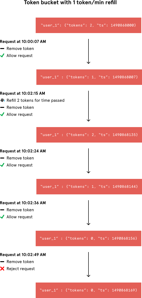
A simple Google search for “rate limit algorithm” points us to the classic token bucket algorithm (or leaky bucket as a meter algorithm). For each unique user, we would record their last request’s Unix timestamp and available token count within a hash in Redis. We would store these two values in a hash rather than as two separate Redis keys for memory efficiency. An example hash would look like this:

Whenever a new request arrives from a user, the rate limiter would have to do a number of things to track usage. It would fetch the hash from Redis and refill the available tokens based on a chosen refill rate and the time of the user’s last request. Then, it would update the hash with the current request’s timestamp and the new available token count. When the available token count drops to zero, the rate limiter knows the user has exceeded the limit.
Despite the token bucket algorithm’s elegance and tiny memory footprint, its Redis operations aren’t atomic. In a distributed environment, the “read-and-then-write” behavior creates a race condition, which means the rate limiter can at times be too lenient.
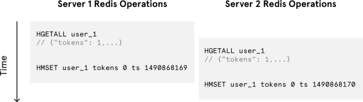
Imagine if there was only one available token for a user and that user issued multiple requests. If two separate processes served each of these requests and concurrently read the available token count before either of them updated it, each process would think the user had a single token left and that they had not hit the rate limit.
Our token bucket implementation could achieve atomicity if each process were to fetch a Redis lock for the duration of its Redis operations. This, however, would come at the expense of slowing down concurrent requests from the same user and introducing another layer of complexity. Alternatively, we could make the token bucket’s Redis operations atomic via Lua scripting. For simplicity, however, I decided to avoid the unnecessary complications of adding another language to our codebase.
Fixed Window
In a fixed window algorithm, a window size of n seconds (typically using human-friendly values, such as 60 or 3600 seconds) is used to track the rate. Each incoming request increments the counter for the window. If the counter exceeds a threshold, the request is discarded. The windows are typically defined by the floor of the current timestamp, so 12:00:03 with a 60 second window length, would be in the 12:00:00 window.

The advantage of this algorithm is that it ensures more recent requests gets processed without being starved by old requests. However, a single burst of traffic that occurs near the boundary of a window can result in twice the rate of requests being processed, because it will allow requests for both the current and next windows within a short time. Additionally, if many consumers wait for a reset window, for example at the top of the hour, then they may stampede your API at the same time.
Link – For example, a rate limiter for a service that allows only 10 requests per an hour will have the data model like below. Here, the buckets are the windows of one hour, with values storing the counts of the requests seen in that hour.
{
 "1AM-2AM": 7,
 "2AM-3AM": 8
}
This in incorrect.
Explanation: In the above case, if all the 7 requests in the 1AM-2AM bucket occurs from 1:30AM-2AM, and all the 8 requests from 2AM-3AM bucket occur from 2AM-2:30AM, then effectively we have 15(7 + 8) requests in the time range of 1:30AM-2:30AM, which is violating the condition of 10req/hr.
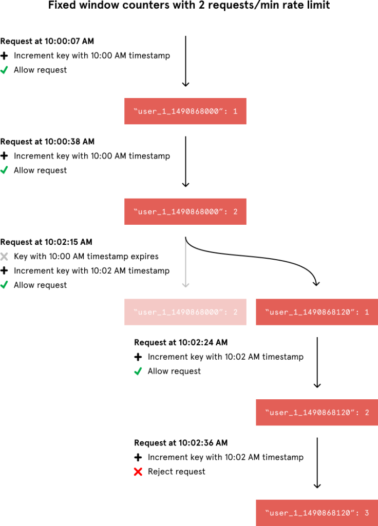
Link When incrementing the request count for a given timestamp, we would compare its value to our rate limit to decide whether to reject the request. We would also tell Redis to expire the key when the current minute passed to ensure that stale counters didn’t stick around forever.

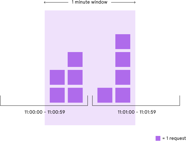
Although the fixed window approach offers a straightforward mental model, it can sometimes let through twice the number of allowed requests per minute. For example, if our rate limit were 5 requests per minute and a user made 5 requests at 11:00:59, they could make 5 more requests at 11:01:00 because a new counter begins at the start of each minute. Despite a rate limit of 5 requests per minute, we’ve now allowed 10 requests in less than one minute!
We could avoid this issue by adding another rate limit with a smaller threshold and shorter enforcement window — e.g. 2 requests per second in addition to 5 requests per minute — but this would overcomplicate the rate limit. Arguably, it would also impose too severe of a restriction on how often the user could make requests.
Sliding window log [Link]
The final rate limiter implementation I considered optimizes for accuracy — it just stores a timestamp for each request. As Peter Hayes describes, we could efficiently track all of a user’s requests in a single sorted set.
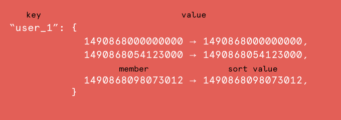
When the web application processes a request, it would insert a new member into the sorted set with a sort value of the Unix microsecond timestamp. This would allow us to efficiently remove all of the set’s members with outdated timestamps and count the size of the set afterward. The sorted set’s size would then be equal to the number of requests in the most recent sliding window of time.
Both this algorithm and the fixed window counters approach share an atomic “write-and-then-read” Redis operation sequence, but the former produces a notable side effect. Namely, the rate limiter continues to count requests even after the user exceeds the rate limit. I was comfortable with this behavior, as it would just extend a ban on a malicious user rather than letting their requests through as soon as the window of time had passed.
While the precision of the sliding window log approach may be useful for a developer API, it leaves a considerably large memory footprint because it stores a value for every request. This wasn’t ideal for Figma. A single rate limit of 500 requests per day per user on a website with 10,000 active users per day could hypothetically mean storing 5,000,000 values in Redis. If each stored timestamp value in Redis were even a 4-byte integer, this would take ~20 MB (4 bytes per timestamp 10,000 users 500 requests/user = 20,000,000 bytes).
This method works perfectly.
Cons
- High memory footprint. All the request timestamps needs to be maintained for a window time, thus requires lots of memory to handle multiple users or large window times
- High time complexity for removing the older timestamps
Sliding window counters [Link]
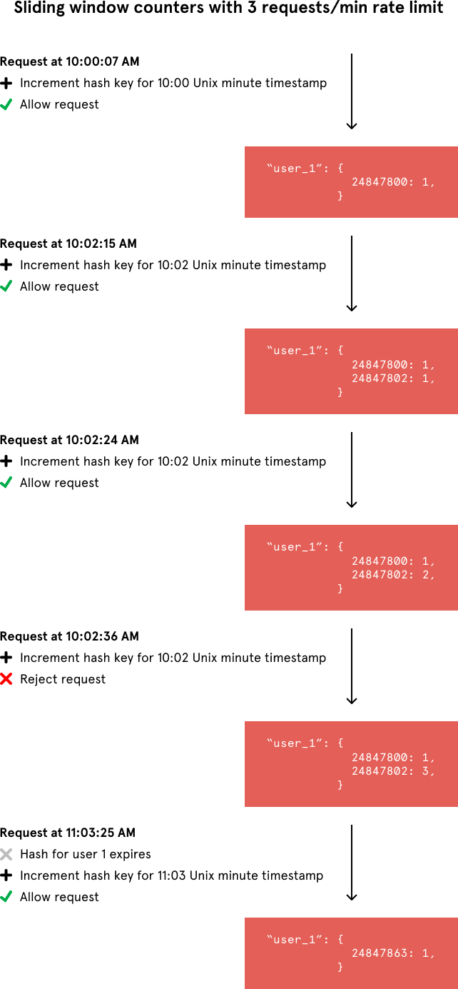
Ultimately, the last two rate limiter approaches — fixed window counters and sliding window log — inspired the algorithm that stopped the spammers. We count requests from each sender using multiple fixed time windows 1/60th the size of our rate limit’s time window.
For example, if we have an hourly rate limit, we increment counters specific to the current Unix minute timestamp and calculate the sum of all counters in the past hour when we receive a new request. To reduce our memory footprint, we store our counters in a Redis hash — they offer extremely efficient storage when they have fewer than 100 keys. When each request increments a counter in the hash, it also sets the hash to expire an hour later. In the event that a user makes requests every minute, the user’s hash can grow large from holding onto counters for bygone timestamps. We prevent this by regularly removing these counters when there are a considerable number of them.
Let’s compare the memory usage of this algorithm with our calculation from the sliding window log algorithm. If we have a rate limit of 500 requests per day per user on a website with 10,000 active users, we would at most need to store ~600,000 values in Redis. That comes out to a memory footprint of ~2.4 MB (4 bytes per counter 60 counters 10,000 users = 2,400,000 bytes). This is a bit more scalable.
- This is a hybrid of Fixed Window Counters and Sliding Window logs
- The entire window time is broken down into smaller buckets. The size of each bucket depends on how much elasticity is allowed for the rate limiter
- Each bucket stores the request count corresponding to the bucket range.
For example, in order to build a rate limiter of 100 req/hr, say a bucket size of 20 mins is chosen, then there are 3 buckets in the unit time
For a window time of 2AM to 3AM, the buckets are
{
 "2AM-2:20AM": 10,
 "2:20AM-2:40AM": 20,
 "2:40AM-3:00AM": 30
}
If a request is received at 2:50AM, we find out the total requests in last 3 buckets including the current and add them, in this case they sum upto 60 (<100), so a new request is added to the bucket of 2:40AM–3:00AM giving…
{
 "2AM-2:20AM": 10,
 "2:20AM-2:40AM": 20,
 "2:40AM-3:00AM": 31
}
Note: This is not a completely correct, for example: At 2:50, a time interval from 1:50 to 2:50 should be considered, but in the above example the first 10 mins isn’t considered and it may happen that in this missed 10 mins, there might’ve been a traffic spike and the request count might be 100 and hence the request is to be rejected. But by tuning the bucket size, we can reach a fair approximation of the ideal rate limiter.
Space Complexity: O(number of buckets)
Time Complexity: O(1) — Fetch the recent bucket, increment and check against the total sum of buckets(can be stored in a totalCount variable).
Pros
- No large memory footprint as only the counts are stored
Cons
- Works only for not-so-strict look back window times, especially for smaller unit times
